
More Information
Submitted: May 21, 2026 | Approved: June 05, 2026 | Published: June 08, 2026
How to cite this article: Pavlenko V, Lukashuk D. Modeling of Eye Movement System Using Orthogonal Visual Stimuli and Volterra Polynomial Representations. J Neurosci Neurol Disord. 2026; 10(1): 25-38. Available from:
https://dx.doi.org/10.29328/journal.jnnd.1001117
DOI: 10.29328/journal.jnnd.1001117
Copyright License: © 2026 Pavlenko V, et al. This is an open access article distributed under the Creative Commons Attribution License, which permits unrestricted use, distribution, and reproduction in any medium, provided the original work is properly cited.
Keywords: Nonlinear integral models; Eye movement system; Eye-tracking; Test visual stimuli; Psychophysiological state; Machine learning; Classification; Bayesian method; Support vector machine

Modeling of Eye Movement System Using Orthogonal Visual Stimuli and Volterra Polynomial Representations
Vitaliy Pavlenko* and Denys Lukashuk
Department of Computerized Systems and Software Technologies, Odesa Polytechnic National University, Shevchenko Avenue 1, Odesa, 65044, Ukraine
*Address for Correspondence: Vitaliy Pavlenko, Department of Computerized Systems and Software Technologies, Odesa Polytechnic National University, Shevchenko Avenue 1, Odesa, 65044, Ukraine, Email: [email protected]
This paper presents an approach to the modeling and diagnostic analysis of the human eye movement system (EMS) based on nonlinear integral models and Volterra polynomial representations in the form of multidimensional transient characteristics. Experimental “input-output” data were obtained using eye-tracking technology during identification experiments with three test visual stimuli positioned at different distances relative to the initial fixation point. The proposed methodology enabled the construction of adequate EMS models that combine high identification accuracy with a relatively simple mathematical representation. Two EMS models were formed from the experimental data: Model1, derived from horizontal experiments, and Model2, obtained from vertical experiments. Diagnostic feature spaces were generated using the transient characteristics of models for further psychophysiological state classification by machine learning methods. Two categories of feature spaces were investigated: heuristic features and features obtained from approximation and detail coefficients produced by wavelet decomposition of EMS transient characteristics. To improve dataset representativeness, augmentation with Gaussian noise levels of 1%, 3%, and 5% was performed. Classification efficiency was evaluated using Stratified K-Fold cross-validation with 8 folds for the original datasets and 32 folds for the augmented datasets. An exhaustive computational search was applied to determine the most informative feature combinations according to the probability of correct recognition (PCR) criterion. Pairwise feature combinations were analyzed for all datasets, whereas triplet combinations were additionally investigated for augmented data. The obtained results indicate that dataset augmentation considerably improves classification performance compared to the original data. In the heuristic feature spaces, the maximum PCR increased from 87.5% for the original datasets to 98.44% after augmentation for feature pairs, while the analysis of triplet combinations on augmented datasets produced PCR values approaching 100% within the applied cross-validation procedure. In the wavelet-based feature spaces, PCR values increased from 68.75% to 85.94% for augmented feature pairs and up to 95.31% for triplet combinations. The obtained findings confirm the effectiveness of the proposed intelligent information technology for psychophysiological state diagnostics based on quadratic Volterra EMS models and machine learning techniques. The proposed approach can be considered a basis for further development of machine learning methods for eye-tracking-based psychophysiological state assessment.
The human eye movement system (EMS) plays a crucial role in neuroscience, medicine, and artificial intelligence, since its parameters provide valuable information about cognitive activity, psychophysiological states, and neurological disorders. Eye-tracking technology, as a non-invasive tool, has been widely employed to investigate these processes and to develop diagnostic and predictive models of human behavior. In this context, accurate modeling of EMS dynamics is of particular importance for both theoretical understanding and practical applications.
A growing body of research has demonstrated the relevance of eye-tracking in the diagnosis of cognitive and neurological impairments. For example, eye movement parameters have been analyzed to characterize Parkinson’s disease [1,2], while eye-tracking biomarkers have been proposed for the diagnosis of autism in primary care [3]. Similarly, specific oculomotor features were studied in the context of dyslexia, contributing to the development of assistive technologies for individuals with reading difficulties [4]. Other studies have focused on the relationship between eye movement parameters, mental workload, and fatigue, showing their applicability for assessing psychophysiological states in professional activities with high cognitive demands [5,6]. Furthermore, machine learning approaches have been applied to predict individual mental states from EMS data, illustrating the potential of combining eye-tracking with artificial intelligence methods [7].
Recent progress in AI-based data analysis has further enhanced the potential of EMS research. Deep learning models have been employed for detecting pathological changes in eye movements and for early diagnosis of neurological disorders [8-10]. Additionally, transfer learning approaches have been utilized to improve the accuracy and generalization of eye-disease detection systems, demonstrating the growing synergy between biomedical signal processing and AI [9].
Another promising direction is the use of nonlinear system identification methods for modeling EMS dynamics. Integral nonlinear models based on Volterra polynomials allow for capturing the inherent nonlinearities of eye movement responses. Prior studies have applied such models for the analysis of neurophysiological signals [11], while Volterra-Laguerre structures have been proposed for the description of smooth pursuit movements [12]. The theoretical foundations of Volterra-based modeling for system identification and control are well established in classical works [13].
In addition to medical and cognitive research, eye-tracking technologies are increasingly applied in broader contexts, including teamwork evaluation in healthcare [14], biometric authentication [15], motor imagery analysis [16], cognitive assessment in education [17], learning analytics [18], brain–computer interface development [19], software engineering tasks [20], and training for vision-intensive professions such as aviation [21]. Recent advances further confirm that eye movement parameters constitute an informative source for assessing psychophysiological and cognitive states, as demonstrated by studies on mental fatigue recognition using deep learning [22], cognitive assessment of patients with disorders of consciousness [23], eye-tracking-based attention training in poststroke rehabilitation [24], and the identification of cognitive and social intention states based on eye gaze parameters and oculomotor behavior [25]. These applications highlight the versatility of EMS analysis, bridging multiple disciplines from medicine to artificial intelligence.
Therefore, EMS research represents a highly interdisciplinary field with wide-ranging applications. In this study, we propose an approach for modeling eye movements using nonlinear Volterra models. The objective is to improve the accuracy of EMS identification and to provide a methodological basis for psychophysiological state assessment and applied developments across medical, cognitive, and engineering domains.
The human EMS reflects essential cognitive and psychophysiological processes, and its modeling provides valuable tools for assessing the functional state of the central nervous system. Conventional approaches to eye movement analysis mainly rely on empirical methods and simplified parametric models, which often fail to capture the nonlinear dynamic properties of the EMS. In contrast, integral nonlinear models, in particular first- and second-order Volterra representations in the form of transient characteristics, have demonstrated significant potential for improving the diagnostic evaluation of psychophysiological states [26].
The objective of the present study is to examine the diagnostic effectiveness of second-order Volterra models of the EMS, obtained from experimental “input-output” eye-tracking data. Unlike previous studies, where test stimuli were applied exclusively in the horizontal direction, the current work expands the experimental design by including both horizontal and vertical trajectories of visual stimulation. This extension enables a more comprehensive assessment of the EMS and allows for analyzing the effect of stimulus direction on the accuracy of psychophysiological state classification.
The subject of investigation comprises computational methods and software tools for extracting diagnostic features from EMS identification data, parameterized as first- and second-order transient characteristics. Particular attention is given to the formation of feature spaces and the construction of classifiers, including Bayesian and Support Vector Machine approaches, with a focus on evaluating how the choice of stimulus direction influences the classification performance.
This research represents a further step in the development of intelligent information technologies for psychophysiological state assessment, advancing earlier approaches by introducing multidirectional EMS identification and systematically studying its impact on diagnostic reliability.
For the identification of the nonlinear dynamic system (NDS), mathematical models in the form of Volterra integro-power polynomials are employed. The least squares method (LSM) [26] is used for EMS identification. In this study, two models are utilized for EMS identification: Model1 and Model2. Model1 is based on horizontal test visual stimuli, whereas Model2 is constructed from orthogonal vertical test experiments.
The time-domain identification method is applied for building Model1, which is based on approximating the response y(t) of the NDS to an input deterministic signal x(t) by an integro‑power polynomial of order N (where N is the order of the approximation model):
(1)
where ŷn(t) denotes the partial components of the model response (with n being the convolution dimension), and
wn(t – τ1,…, t – τn) is the Volterra kernel of order n.
The following statement holds [26].
Statement. Let the test signals a1x(t), a2x(t), …, aLx(t) be sequentially applied to the input of the NDS; L ≥ N a1, a2,…, aL are distinct real numbers satisfying the condition 0< aj ≤1, for ∀j=1,2,..., L; and x(t) is a deterministic signal. Then:
(2)
The partial components in the approximation model are determined using the LSM. This makes it possible to obtain such estimates, for which the sum of squared deviations of the responses of the identified NDS y(aj x(t)) = y(t | aj) from the responses of the model is minimized, i.e., it ensures the minimum of the mean square error criterion. The minimization of the criterion reduces to solving the system of Gauss normal equations, which can be written in vector-matrix form as:
, (3)
where
and denotes the transposed matrix.
From equation (3), we obtain
, (4)
If step test signals with amplitudes a1, a2,…, aL are applied to the input of the system to be identified, the estimates of the transient characteristics and diagonal cross-sections of the NDS transient characteristics, …, are obtained [26].
The responses of the investigated EMS models in the general case are computed based on the expression:
(5)
or
(6)
Model2, based on vertical orthogonal data, is constructed analogously to Model1.
The test signals b1u(t), b2u(t), …, bLu(t) are applied sequentially to the input of the NDS, where b1, b2,…,bL (L ≥ N) are distinct real numbers satisfying the condition 0< bj ≤1, for ∀j=1,2,..., L; and u(t) is an input deterministic signal.
The partial components in the approximation model are determined using the LSM, ensuring that the sum of squared deviations of the responses of the identified NDS z(bj u(t)) = z(t | bj) from the responses of the model is minimized. The minimization of the criterion reduces to solving the system of Gauss normal equations, which can be written in vector-matrix form as:
, (7)
where
and denotes the transposed matrix.
From equation (6), we obtain
. (8)
If step test signals with amplitudes b1, b2,…,bL are applied to the input of the system to be identified, the estimates of the transient characteristics and diagonal cross-sections of the NDS transient characteristics ,… are obtained in the same way as in Model1.
The responses of the EMS model, based on Model2, are computed using the expression:
(9)
or
(10)
The problem of accuracy evaluation of EMS models based on Volterra series was previously investigated in [26], where three model orders and identification methods were compared. In the present study, the analysis is focused on the quadratic Volterra model identified by the LSM using step test signals of different amplitudes. The EMS response to test step signals of the form х(t)=ajθ(t), j=1, 2, 3, where θ(t) denotes the Heaviside function, is analyzed with amplitudes aj (j=1, 2, 3): a1=(1/3)lx, a2=(2/3)lx, a3=lx (lx denotes the screen width of a computer monitor in pixels) was investigated in the context of constructing Volterra models (for higher model accuracy, additional test signals, e.g., 4, 5 or more, can also be used).
For vertical experiments, analogous EMS responses to test step signals are defined as u(t)=bkθ(t) with amplitudes bk (k=1, 2, 3): b1=(1/3)ly, b2=(2/3)ly, b3=ly, where ly denotes the screen height in pixels. The application of such test signals allows obtaining first-order transient functions and only the diagonal sections of higher-order EMS transient functions, as follows from the interpretation of the identification algorithm using the specified test stimuli (5), (6), (9), (10).
For clarity, models derived from horizontal data are denoted as Model1, and those from vertical data as Model2.
For EMS identification, empirical data were obtained in “input-output” experiments using advanced eye-tracking technology. The Tobii Pro TX300 eye tracker was employed to record ocular responses to orthogonal step visual stimuli, presented separately along horizontal and vertical axes. Measurements were carried out at different times of the day, including “Morning” (before work) and “Evening” (after work), as well as on different days [27]. Each complete EMS research cycle for a single participant included three experiments with test signals of increasing amplitude, performed sequentially along each axis.
During each EMS research cycle, the participant initially fixates on the starting position (red point). After a short delay (1-2 sec), the red point disappears, and a test stimulus (blue point) is presented (2-3 sec) at the first test amplitude along the corresponding axis. The red fixation point then reappears, allowing the participant to return their gaze to the initial position. The same procedure is then repeated for the second and third test amplitudes, each separated by a brief interstimulus interval.
The horizontal experiment sequence is illustrated in Figure 1, which shows the initial fixation and successive presentations of the test stimulus at increasing horizontal positions. The corresponding raw eye-tracking signals for horizontal displacements are presented in Figure 2 for the “Morning” and “Evening” conditions.
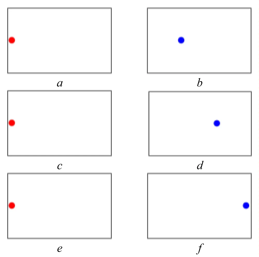
Figure 1: Test stimulus: a), c), e) – initial position; b) – test stimulus position (a1 = 1/3); d) – test stimulus position (a2 = 2/3); f) – test stimulus position (a3 = 1); Source: created by the authors.
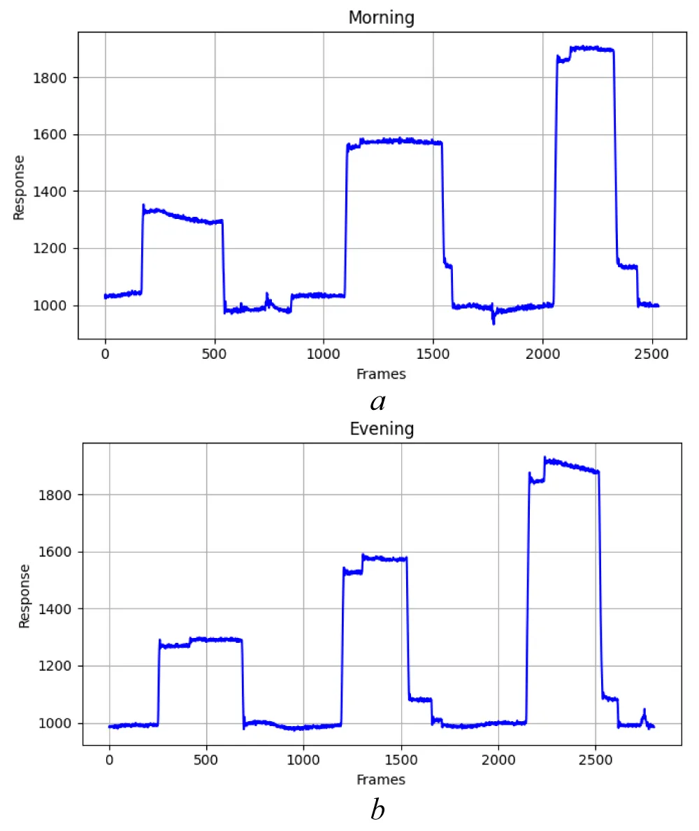
Figure 2: Raw eye tracker output signals recorded during horizontal experiments for the respondent’s state: a) “Morning”, b) “Evening” Source: created by the authors.
It should be noted that the recorded eye movements correspond specifically to saccades, i.e., rapid, ballistic movements of the eye that shift the point of fixation from one target to another. Other types of ocular movements, such as smooth pursuit, were not considered in the current experimental setup. Both horizontal and vertical experiments were conducted sequentially within the same session to ensure consistent physiological and attentional conditions for the participant.
The vertical experiment follows an analogous procedure, with stimuli presented from the top toward the bottom of the screen. The initial fixation and successive vertical positions of the test stimulus are illustrated in Figure 3, and the corresponding raw eye-tracking signals are shown in Figure 4 for the “Morning” and “Evening” conditions.
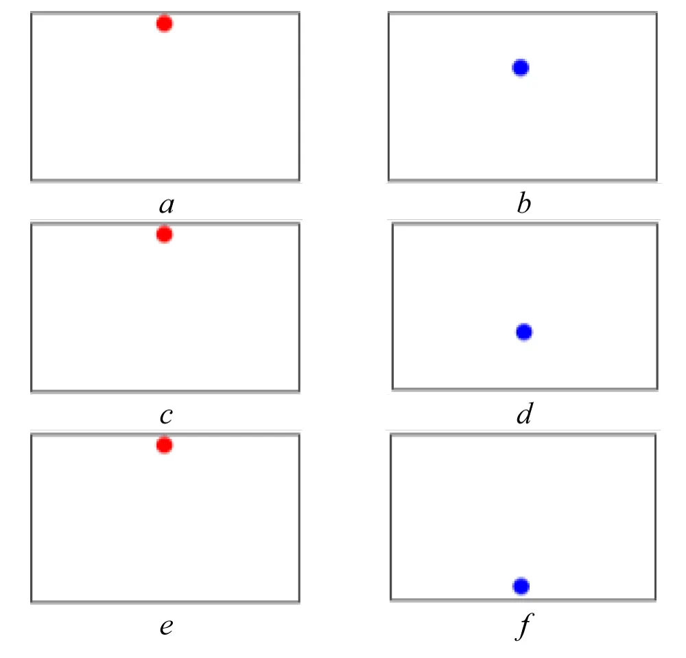
Figure 3: Test stimulus: a), c), e) – initial position; b) – test stimulus position (b1 = 1/3); d) – test stimulus position (b2 = 2/3); f) – test stimulus position (b3 = 1); Source: created by the authors.
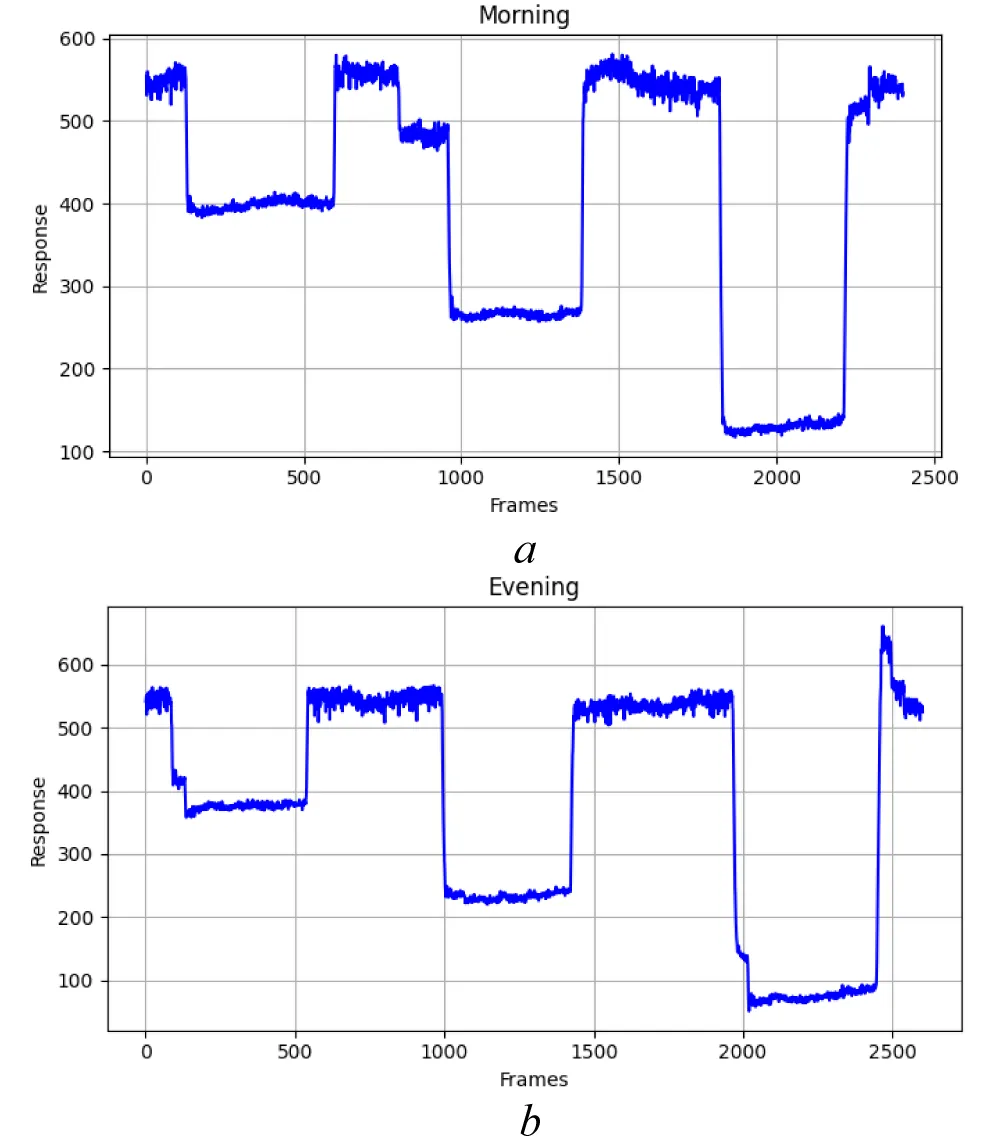
Figure 4: Eye tracker output signals for the respondent’s state: a) “Morning”, b) “Evening”; Source: created by the authors.
This section investigates the specifics of applying empirical data to construct EMS models and evaluates the variability of averaged transient characteristics depending on the psychophysiological state of the subject in the “Morning” and “Evening” conditions. In accordance with the identification algorithm (3), all EMS response data were aligned to a common initial point (synchronization was performed).
The empirical data obtained from horizontal experiments are designated as Dataset1, while those from vertical experiments are designated as Dataset2. Dataset1 comprises eight observations corresponding to the “Morning” state and eight observations corresponding to the “Evening” state, as illustrated in Figure 5. Dataset2 comprises seven observations for the “Morning” state and eight observations for the “Evening” state.
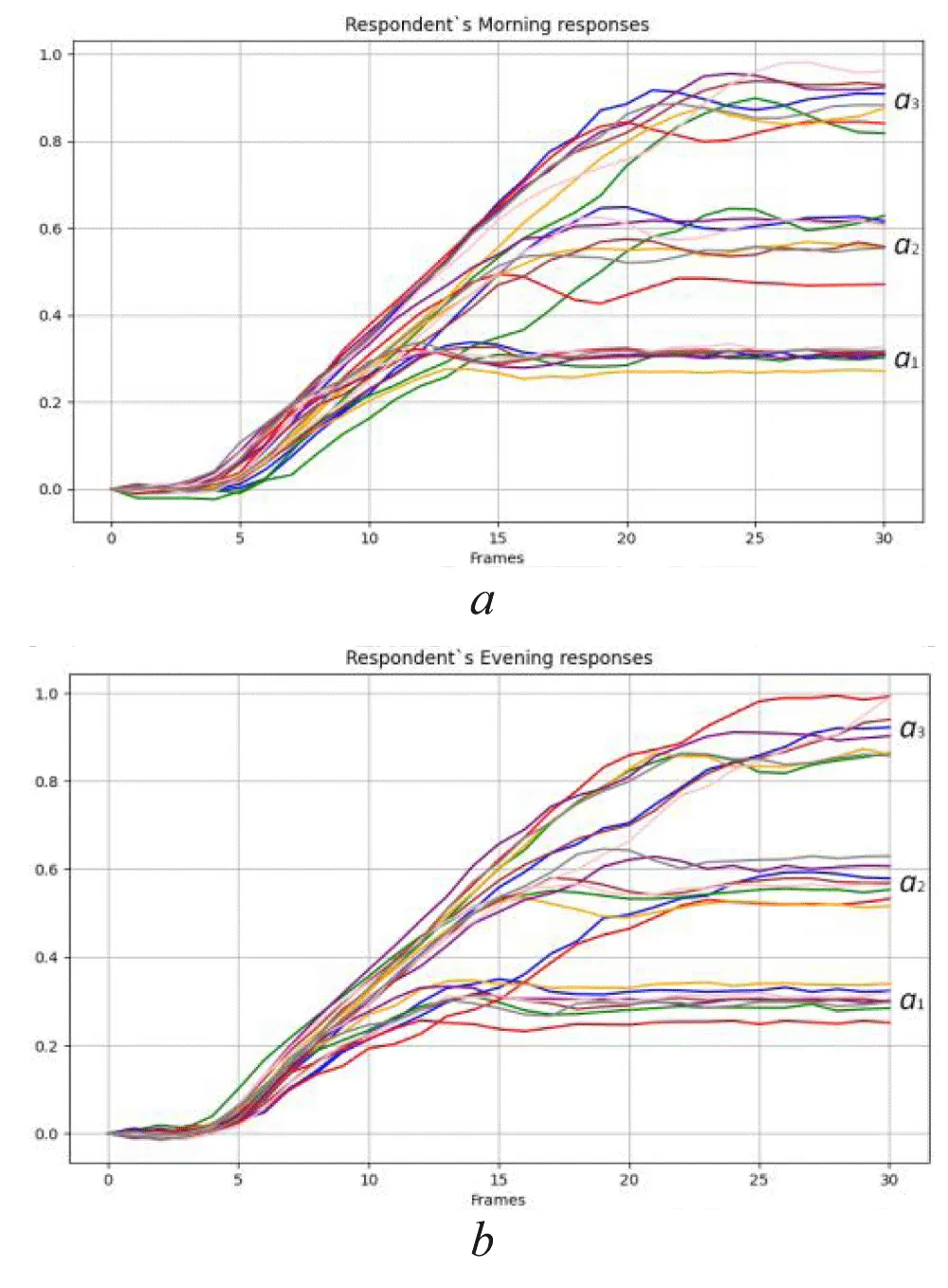
Figure 5: Dataset1 – Empirical eye movement responses in the horizontal direction for the states: a) “Morning”; b) “Evening.” Source: created by the authors.
To increase the dataset diversity and ensure the stability of further statistical analysis, additional synthetic data were generated based on seven real experimental observations using a Variational Autoencoder (VAE) model implemented in Python with the TensorFlow and Keras libraries. The algorithm encoded empirical EMS responses into a low-dimensional latent space and then reconstructed new samples through probabilistic decoding. This approach preserved the nonlinear temporal dynamics of the original eye movement signals while introducing controlled variability. The generated signals were constrained to start from zero and normalized within the range [0, 1], maintaining consistency with the physical characteristics of the real data. For visual comparison, one representative VAE-generated synthetic response is shown in Figure 6a using a dashed line, while the remaining curves correspond to real experimental observations. The vertical experimental data are presented in Figure 6.
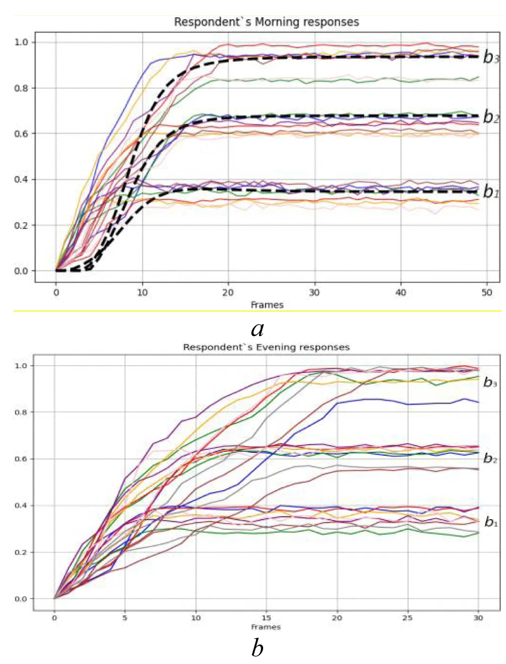
Figure 6: Dataset 2 – Empirical eye Movement responses in the vertical direction for the states: a) “Morning” (the dashed curve denotes a representative VAE-generated synthetic sample); b) “Evening.” Source: created by the authors.
EMS models Model1 and Model2 were constructed separately based on horizontal and vertical experimental data. The transient characteristics derived from the Dataset1 are denoted as and while those obtained from the Dataset2 are denoted as and. The corresponding functions of the first and second orders are presented in Figure 7 and Figure 8, respectively, together with their averaged values in the “Morning” and “Evening” states.
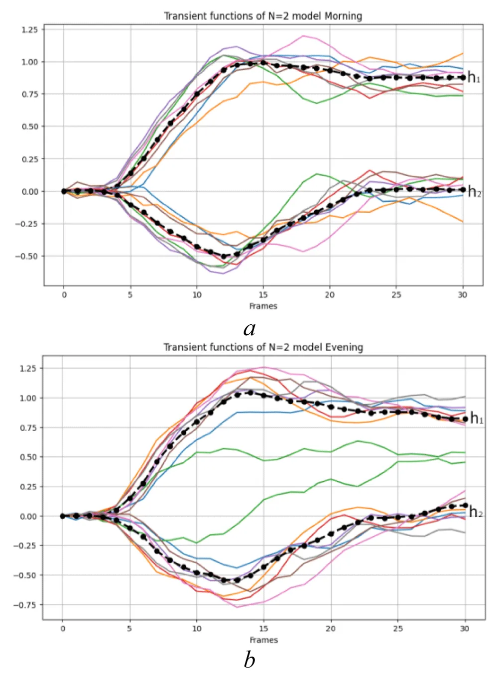
Figure 7: Transient characteristics of the first- and second-order EMS Model 1 obtained from Dataset1 and their averaged values in the states: a) “Morning”; b) “Evening.” Source: created by the authors.
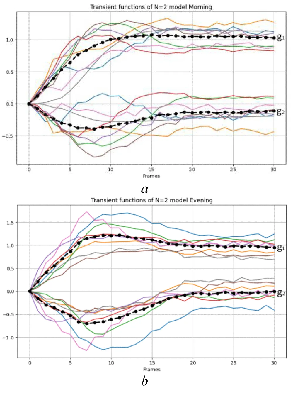
Figure 8: Transient characteristics of the first- and second-order of the EMS Model2 obtained from Dataset2 and their averaged values in the states: a) “Morning”; b) “Evening”; Source: created by the authors.
The variability (deviation) of the averaged transient characteristics of the EMS models Model1 for the respondent’s “Morning” and “Evening” conditions was evaluated using the following metrics:
σnN – maximum deviation
(11)
εnN – normalized root mean square deviation (NRMSD)
(12)
where n = 1,2,…,N.
Using the transient characteristics of Model2, the metrics can be formally represented in the same form as formulas (11) and (12) by considering the “Morning” and “Evening” conditions.
The variability metrics of the averaged transient characteristics for Model1 and Model2 are presented in Table 1.
| Table 1: Variability indicators of the averaged transient characteristics for Model1 and Model2 Source: created by the authors | ||||
| Model | ε1N | σ1N | ε2N | σ2N |
| Model1 | 0.045 | 0.0706 | 0.2444 | 0.0796 |
| Model2 | 0.1257 | 0.3209 | 0.7174 | 0.3226 |
In this work, machine learning techniques are employed to evaluate the efficiency of feature spaces derived from linear and quadratic transient characteristics for the classification of psychophysiological states.
To facilitate further analysis, the following designations are used:
E0 – a feature space composed of heuristic parameters extracted from EMS Model1;
Ẽ0 – a feature space composed of heuristic parameters extracted from the EMS Model2;
W – a feature space obtained from approximation and detail coefficients produced by wavelet decomposition of the Model1 transient characteristics;
W̃ – a feature space obtained from approximation and detail coefficients produced by wavelet decomposition of the Model2 transient characteristics.
Feature spaces E0 and Ẽ0
The heuristic feature space E0 is constructed using transient characteristics of the second-order Volterra model. The choice of these heuristic parameters is justified by earlier research, which demonstrated both informativeness and sensitivity to variations in the subject’s psychophysiological condition. The list of EMS heuristic features derived from the Model1 represents a subset of the features investigated in [26].
In the present study, the subset of heuristic features is grouped into four functional categories depending on their mathematical interpretation and the transient characteristic from which they are derived.
Group 1 – Integral features:
; (13)
. (14)
Group 2 – Features corresponding to the argument and value at the maximum derivative of transient characteristics:
; (15)
; (16)
; (17)
. (18)
Group 3 – Features corresponding to the argument and value at the minimum derivative of transient characteristics:
; (19)
; (20)
; (21)
. (22)
Group 4 – Features corresponding to the argument and value at the maximum transient response:
; (23)
; (24)
; (25)
. (26)
Here, and represent the first- and second-order transient characteristics of the EMS, and their derivatives are denoted by and, respectively.
The feature space Ẽ0 is formed analogously to E0, following the same definitions provided above, with the first- and second-order transient characteristics of Model2 substituted for the corresponding Model1 characteristics. The list of EMS heuristic features derived from the Model2 represents a subset of the features .
Feature spaces W and W̃
The W feature space is generated through wavelet decomposition [28,29] of the transient characteristics of the first and second orders. The decomposition is performed using the discrete wavelet transform (DWT), where Coiflet 4 serves as the mother wavelet with a decomposition level of 2. The feature vector is formed from the first five approximation coefficients (ca) together with the first five detail coefficients (cd) obtained at the second decomposition level. Each feature in the W space is denoted as ,
where w1 = ca[1], …, w5=ca[5], w6 = cd[1],…, w10=cd[5]; m is the feature index corresponding to the selected wavelet coefficients.
For Model1, the features of the feature space W are denoted as wm, whereas for Model2, the corresponding features of the feature space W̃ are denoted as w̃m.
To assess the psychophysiological state of a person, a Bayesian classifier based on experimental EMS data was developed. The classification procedure was implemented using the Gaussian Naïve Bayes (GaussianNB) algorithm from the scikit-learn library in Python.
Given the limited size of the dataset, the Stratified K-Fold cross-validation technique was applied to provide a statistically balanced evaluation while preserving class proportions within each fold. The procedure was used to assess the stability of classification results obtained for the most informative feature combinations identified within the predefined feature spaces. It should be noted that the available experimental data were obtained from repeated measurements of a single respondent, and no independent external test set was available. Therefore, the reported PCR values should be interpreted as indicators of the internal validation performance of the proposed methodology rather than as estimates of population-level generalization capability. For the best-performing feature combinations, 95% confidence intervals (CI) were additionally estimated from the cross-validation results using Student’s t-distribution.
The classification procedure was carried out in specially formed feature spaces E0, Ẽ0, W, and W̃. The evaluation of classification efficiency relied on analyzing the informativeness of different feature combinations using the probability of correct recognition (PCR) criterion. An exhaustive search strategy was applied to systematically evaluate all possible feature pairs and identify the most diagnostically informative combinations.
Original dataset (8-Fold Cross Validation)
At the first stage of the study, classification was performed using the original dataset. The experimental data were divided into 8 stratified folds to ensure a balanced representation of both classes within each validation subset.
Dataset based on Model1: Feature space E0: For the dataset based on Model1, the Bayesian classifier demonstrated a maximum probability of correct recognition of 87.5% for the feature pair:
. (27)
Feature space W: In the wavelet-based feature space W, the classification accuracy was 68.75%, which indicates a lower discriminative capacity compared to the heuristic features.
Dataset based on Model2: Feature space Ẽ0: For Model2, the maximum PCR in the heuristic feature space Ẽ0 reached 75%, which is lower than the corresponding result obtained for Model1.
Feature space W̃: In the wavelet feature space W̃, the achieved PCR was 68.75%, remaining consistent with the result obtained for the analogous wavelet-based space W and indicating limited discriminative capacity.
Dataset based on Model1 and Model2: Feature spaces E0 and Ẽ0: When combining the datasets from Model1 and Model2, the joint heuristic feature spaces E0 and Ẽ0 provided a maximum PCR of 87.5%, matching the highest value obtained for Model1. The following feature pairs yielded this result:
; (28)
; (29)
. (30)
Feature spaces W and W̃: In the combined wavelet feature spaces W and W̃, the classifier achieved a PCR of 68.75%, which is comparatively low and not suitable for reliable classification.
The positioning of training dataset objects in the combined heuristic feature spaces E0 and Ẽ0 for the feature pair e4&ẽ4 is shown in Figure 9.
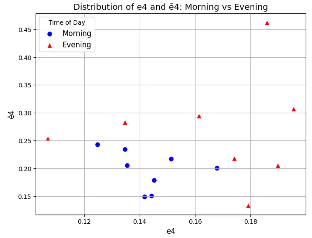
Figure 9: Distribution of training dataset objects e4&ẽ4 in combination with heuristic feature spaces E0 and Ẽ0 ; Source: created by the authors.
Augmented dataset (32-Fold Cross Validation)
For the second stage of the study, the original EMS datasets were augmented by additive Gaussian noise at levels of 1%, 3%, and 5%. This procedure increased the effective size of the training datasets, allowing for more robust evaluation of classifier performance. In connection with the augmented dataset, the number of cross-validation folds was increased to 32 to maintain statistically balanced subsets. The expansion of the dataset also made it possible to investigate not only feature pairs but also feature triplets, which provided a deeper analysis of multidimensional relationships among heuristic and wavelet-based features.
The augmented datasets were used to investigate the influence of increased data variability on classification performance. Although the generated samples preserved the dynamic properties of the original EMS responses and improved the stability of classifier evaluation, they were derived from the original recordings and therefore cannot be regarded as fully independent observations. Consequently, the obtained results should be interpreted as evidence of the robustness of the proposed methodology under controlled augmentation conditions.
Dataset based on Model1: Feature space E0: For Model1, the maximum PCR in the heuristic feature space E0 reached 93.75% for the following feature pair:
. (31)
Feature space W: In the wavelet-based feature space W, the classifier achieved a PCR of 85.94% for the feature pair w2&w8, demonstrating improved accuracy compared to the original dataset.
Dataset based on Model2: Feature space Ẽ0: For Model2, the maximum PCR in the heuristic feature space Ẽ0 reached 87.5% for the feature pair:
. (32)
A slightly lower PCR of 85.94% was obtained for the feature pair:
. (33)
Feature space W̃: In the wavelet-based feature space W̃, the achieved PCR was 81.25% for the feature pair w̃5&w̃8.
Dataset based on Model1 and Model2: Feature spaces E0 and Ẽ0: When combining the augmented datasets from Model1 and Model2, the joint heuristic feature spaces E0 and Ẽ0 provided a noticeable improvement in classification accuracy compared to the individual models. A maximum PCR of 98.44% (95% CI: 95.25-100.00%) was obtained for the feature pair:
. (34)
A PCR of 96.88% was achieved for the feature pair:
. (35)
Feature spaces W and W̃: In the combined wavelet feature spaces W and W̃, the classifier reached a PCR of 85.94% for the feature pair w1&w̃8, which is comparable to the PCR obtained for the horizontal Dataset1 alone. This indicates that, unlike heuristic features, combining horizontal and vertical datasets does not lead to an improvement in classification accuracy for wavelet-based features.
The positioning of training dataset objects in the combined heuristic feature spaces E0 and Ẽ0, reflecting the impact of 1, 3, and 5% noise levels for the feature pair e12&ẽ4, is shown in Figure 10.
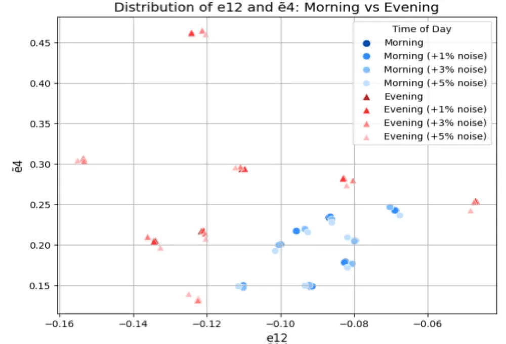
Figure 10: Distribution of training dataset objects e12&ẽ4, reflecting the impact of 1, 3, and 5% noise in combination with heuristic feature spaces E0 and Ẽ0; Source: created by the authors.
Feature Triplet Analysis: The availability of the augmented dataset enabled the examination of feature triplets, allowing for the identification of more complex diagnostic relationships. The results obtained for three-feature combinations in all six feature spaces are summarized below.
Feature space E0: For the heuristic feature space constructed from Model1, the highest PCR value of 93.75% was achieved for feature triplets: e1&e5&e12, e2&e5&e11, e2&e5&e12, e5&e11&e12, and e5&e12&e17.
Feature space Ẽ0: For the vertical Model2, the highest PCR of 96.88% was obtained for the triplet ẽ4&ẽ13&ẽ19, while PCR of 93.75% was achieved for the combination ẽ12&ẽ13&ẽ17, indicating slightly better discriminative potential compared to the horizontal Model1.
Feature spaces E0 and Ẽ0: When merging the heuristic feature spaces, a nearly perfect classification performance (PCR ≈ 100%) was achieved for several combinations, including:
(36)
(37)
A PCR of 98.44% (95% CI: 95.25-100.00%) was recorded for the triplets e1&e12&ẽ4 and e12&ẽ12&ẽ13, confirming the synergistic improvement resulting from the joint use of horizontal and vertical heuristic features.
Feature space W: For the wavelet-based space W, the triplets w1&w2&w8 and w1&w7&w8 provided the maximum PCR of 81.25%, which is lower than the corresponding results obtained in the heuristic feature domain.
Feature space W̃: For Model2, the triplet w̃2&w̃4&w̃7 achieved the highest PCR of 85.94%, while combinations such as w̃2&w̃7&w̃8 yielded 81.25%. These results indicate a consistent yet moderate improvement compared with the pairwise feature configurations.
Feature spaces W and W̃: When combining the horizontal and vertical wavelet feature spaces, the classifier reached a maximum PCR of 95.31% (95% CI: 89.97-98.84%) for the triplet w1&w̃7&w̃8. Slightly lower results (PCR = 93.75%) were obtained for the triplets w1&w̃1&w̃4 and w1&w̃2&w̃4, demonstrating a limited but measurable benefit from the integration of the two wavelet domains, though the accuracy remains lower than that observed in the heuristic feature spaces.
The summarized results of all experiments with the Bayesian classifier are presented in Table 2. The table compares the maximum PCR values obtained using the original and augmented datasets across different feature spaces.
| Table 2. Maximum PCR values obtained using the Bayesian classifier for original and augmented data in heuristic and wavelet-based feature spaces, % Source: created by the authors |
|||
| Original | Augmented (pairs) | Augmented (triplets) | |
| 87.5 | 93.75 | 93.75 | |
| 75 | 87.5 | 96.88 | |
The comparative visualization of these results is shown in Figure 11 as a bar chart, which clearly illustrates the effect of data augmentation on the classifier’s performance in different feature spaces.
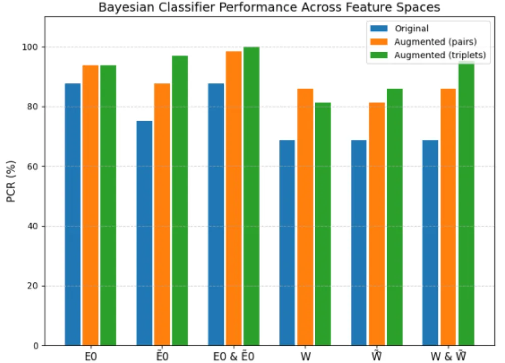
Figure 11: Comparison of maximum PCR values obtained using the Bayesian classifier for original and noise-augmented datasets (pairwise and triplet feature configurations) Source: created by the authors.
To further assess the potential of the feature spaces in classifying psychophysiological states, a support vector machine (SVM) classifier with a Gaussian (RBF) kernel was implemented. The classifier was trained and evaluated in the Python environment using the sklearn.svm.SVC class from the Scikit-learn library. Classification performance metrics were calculated using functions from the sklearn.metrics module. Given the limited size of the datasets, Stratified K-Fold cross-validation was applied to provide a statistically balanced evaluation of the classifier performance, with fold numbers corresponding to the dataset type (8-fold for original and 32-fold for augmented datasets).
For the best-performing feature combinations, 95% confidence intervals were estimated from the cross-validation results using Student’s t-distribution.
Original dataset (8-Fold Cross Validation)
At this stage, classification was performed using the original dataset. The results for individual EMS models and their combination are summarized below.
Dataset based on Model1: Feature space E0: For Model1, the SVM classifier achieved a maximum PCR of 81.25% for the following feature pairs:
; (38)
. (39)
Feature space W: In the wavelet feature space W, the maximum PCR was 75% for the feature pairs: w7&w8 and w8&w9.
Dataset based on Model2: Feature space Ẽ0: For Model2, the maximum PCR in the heuristic feature space Ẽ0 reached 81.25% for the feature pairs:
; (40)
. (41)
Feature space W̃: In the wavelet feature space W̃, the achieved PCR was 68.75%.
Dataset based on Model1 and Model2: Feature spaces E0 and Ẽ0: When combining the original datasets from Model1 and Model2, the joint heuristic feature spaces E0 and Ẽ0 provided a maximum PCR of 81.25% for the following feature pairs:
; (42)
; (43)
; (44)
; (45)
; (46)
. (47)
The positioning of training dataset objects in the combined heuristic feature spaces E0 and Ẽ0 for the feature pair e6&ẽ4 is shown in Figure 12.
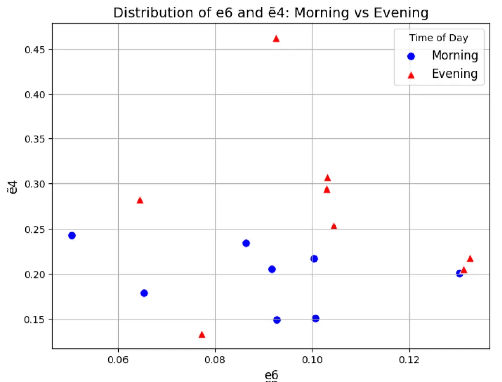
Figure 12: Distribution of training dataset objects e12&ẽ4 in combination of heuristic feature spaces E0 and Ẽ0 ; Source: created by the authors.
Feature spaces W and W̃: In the combined wavelet feature spaces W and W̃, the maximum PCR was 75% for the feature pair w1&w̃4, showing that combining datasets does not substantially improve classification accuracy for wavelet-based features under the original dataset conditions.
Augmented dataset (32-Fold Cross Validation)
For this stage, the datasets were expanded by adding Gaussian noise at 1%, 3%, and 5% levels. Consequently, the number of cross-validation folds was increased to 32 to maintain statistical balance and provide a more reliable estimate of classifier performance.
Dataset based on Model1: Feature space E0: The SVM classifier achieved a maximum PCR of 85.94% for the feature pair:
(48)
Feature space W: In the wavelet space W, the maximum PCR reached 87.5% for the feature pair w4&w8.
Dataset based on Model2: Feature space Ẽ0: For Model2, the heuristic feature space Ẽ0 yielded a maximum PCR of 93.75% for the feature pairs:
; (49)
. (50)
Feature space W̃: In the wavelet space W̃, the classifier reached a PCR of 89.06% for the feature pair w̃7&w̃9, while a PCR of 87.5% was observed for the pairs w̃1&w̃3, w̃7&w̃8.
Dataset based on Model1 and Model2: Feature spaces E0 and Ẽ0: Combining the augmented datasets from Model1 and Model2 led to a substantial improvement in classification performance for heuristic features. A maximum PCR of 98.44% (95% CI: 95.25-100.00%) was obtained for the feature pairs:
; (51)
. (52)
The positioning of training dataset objects in the combined heuristic feature spaces E0 and Ẽ0, reflecting the impact of 1, 3,
and 5% noise levels for the feature pair e12&ẽ12, is shown in Figure 13.
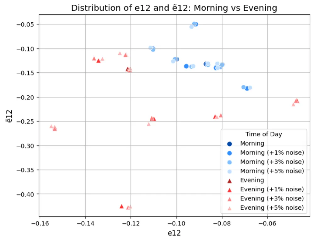
Figure 13: Distribution of training dataset objects e12&ẽ12, reflecting the impact of 1, 3, and 5% noise in combination with heuristic feature spaces E0 and Ẽ0; Source: created by the authors.
Feature space W and W̃: In the combined wavelet feature spaces W and W̃, the SVM classifier achieved a PCR of 89.06% for the feature pair w2&w̃5, demonstrating a modest improvement compared to individual models. Unlike heuristic features, combining datasets for wavelet-based features provides only a moderate gain in classification accuracy.
Feature triplet analysis: The expansion of the dataset through augmentation made it possible to analyze three-feature combinations and evaluate their contribution to classification performance.
Feature space E0: For the heuristic space based on Model1, the highest PCR of 84.38% was achieved for the triplet e1&e7&e11, while a slightly lower value of 82.81% was obtained for e4&e10&e12.
Feature space Ẽ0: For Model2, the top PCR of 93.75% was achieved for several triplets, including ẽ4&ẽ13&ẽ18, ẽ6&ẽ13&ẽ18, ẽ10&ẽ13&ẽ18, ẽ12&ẽ13&ẽ18, and ẽ13&ẽ16&ẽ18.
Feature spaces E0 and Ẽ0: When merging the heuristic feature spaces, the classifier reached a maximum PCR of 93.75% (95% CI: 87.69-96.66%) for multiple triplets, such as:
(53)
(54)
(55)
Slightly lower results (PCR = 92.19%) were obtained for e12&ẽ6&ẽ10, while the feature pairs provided higher classification accuracy.
Feature space W: In the wavelet-based space, the maximum PCR of 87.5% was achieved for several triplets, including w4&w6&w8, w4&w7&w8, w4&w8&w9, w4&w8&w10, w6&w8&w9, and w6&w8&w10.
Feature space W̃: For Model2, the triplet w̃7&w̃8&w̃9 yielded the highest PCR of 93.75%, while w̃1&w̃3&w̃5 produced 89.06%.
Feature spaces W and W̃: When combining the horizontal and vertical wavelet feature spaces, the classifier reached a maximum PCR of 95.31% (95% CI: 89.97-98.84%) for w8&w̃7&w̃8, with w4&w8&w̃7 showing a slightly lower value of 93.75%. This performance exceeds the best result obtained for the pairwise wavelet feature combinations (PCR = 89.06%), indicating an additional gain from incorporating a third complementary feature [28-30] .
The summarized results of all experiments with the SVM classifier, including original and augmented data, are presented in Table 3.
| Table 3. Maximum PCR values obtained using the Bayesian classifier for original and augmented data in heuri©©stic and wavelet-based feature spaces, % Source: created by the uthors | |||
| Feature space | Original | Augmented (pairs) | Augmented (triplets) |
| E0 | 81.25 | 85.94 | 84.38 |
| Ẽ0 | 81.25 | 93.75 | 93.75 |
| E0 & Ẽ0 | 81.25 | 98.44 | 93.75 |
| W | 75 | 87.5 | 87.5 |
| W̃ | 68.75 | 89.06 | 93.75 |
| W & W̃ | 75 | 89.06 | 95.31 |
The comparative visualization of these results is shown in Figure 14.
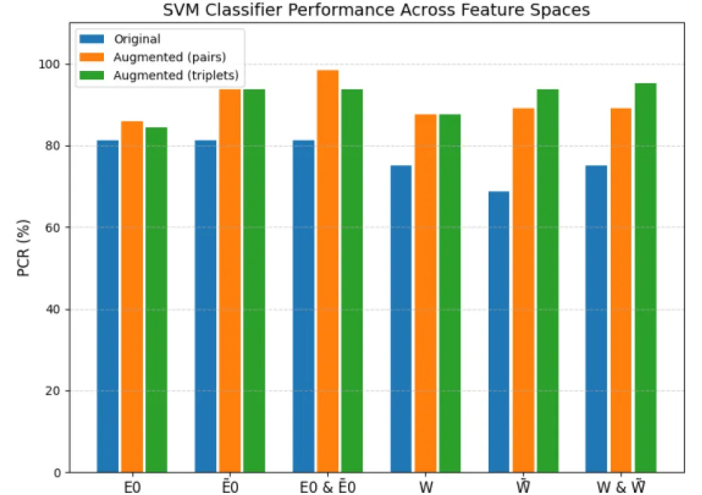
Figure 14: Comparison of maximum PCR values obtained using the SVM classifier for original and noise-augmented datasets (pairwise and triplet feature configurations) Source: created by the authors.
To complement the PCR analysis, additional SVM performance metrics, including Recall, Precision, and F1-score, were calculated for the most informative feature combinations. The results are presented in Table 4.
| Table 4. Performance metrics of the SVM classifier for the most informative heuristic and wavelet feature combinations. Source: created by the authors | ||||
| Metric | e12&ẽ10 | e6&ẽ13&ẽ18 | w2&w̃5 | w̃7&w̃8&w̃9 |
| PCR | 0.9844 | 0.9375 | 0.8906 | 0.9375 |
| Recall | 0.9844 | 0.9375 | 0.8906 | 0.9375 |
| Precision | 0.9766 | 0.9062 | 0.8359 | 0.9062 |
| F1-Score | 0.9792 | 0.9139 | 0.8542 | 0.9167 |
In this study, the human eye movement system was investigated using nonlinear integral models represented by quadratic Volterra polynomials in the form of multidimensional transient characteristics. Experimental “input-output” data were obtained with the help of advanced eye-tracking technology, enabling the identification of EMS models based on three test signals of different amplitudes. This approach ensured adequate accuracy while maintaining the simplicity of the mathematical description of the system.
Diagnostic feature spaces were constructed based on the transient characteristics of the EMS models. The informativeness of the heuristic feature space (E0 and Ẽ0) and the feature space (W and W̃) formed on the basis of wavelet decomposition coefficients was analyzed. To assess the human psychophysiological state, statistical machine learning methods were applied within these diagnostic spaces. Training datasets were formed for two experimental orientations: horizontal (Model1) and vertical (Model2) eye movements, as well as for a combined dataset integrating both orientations.
To improve representativeness and generalization, dataset augmentation was performed by adding Gaussian noise at levels of 1%, 3%, and 5%. This procedure expanded the available data and allowed the analysis of both feature pairs and triplets. Classifier performance was evaluated using Stratified K-Fold cross-validation to ensure class balance, applying 8 folds to the original datasets and 32 folds to the augmented ones. An exhaustive computer-based search of feature combinations identified pairs and triplets with the maximum probability of correct recognition (PCR).
A key novelty of this work lies in the integrated experimental design, which includes classification not only for horizontal and vertical datasets separately but also for their combined version. This approach made it possible to analyze the influence of experimental orientation on recognition reliability and to evaluate the contribution of feature combinations derived from integrated models to diagnostic performance.
The results demonstrate the influence of dataset augmentation and the obtained two- and three-feature combinations on classification efficiency. For the Bayesian classifier, using the original heuristic feature pairs derived from Model1 yielded a maximum PCR of 87.5%, from Model2 – 75%, and from the combined dataset based on both models – 87.5%. After dataset augmentation, PCR increased to 93.75% for Model1, 87.5% for Model2, and 98.44% for the combined dataset.
In the wavelet-based spaces, the maximum PCR for original feature pairs was 68.75% for all individual and combined datasets, while augmentation improved the results to 85.94% for Model1, 81.25% for Model2, and 85.94% for the combined dataset.
Analysis of feature triplets further enhanced recognition performance, achieving PCR values of 93.75% (Model1), 96.88% (Model2), and 100% for the combined dataset in heuristic spaces, and 81.25%, 85.94%, and 95.31% in wavelet-based spaces, respectively.
SVM classifiers generally demonstrated lower reliability compared to the Bayesian approach. For heuristic feature pairs, the maximum PCR was 81.25% for Model1, Model2, and the combined dataset. After augmentation, these values increased to 85.94% (Model1), 93.75% (Model2), and 98.44% (combined). In the wavelet-based spaces, pairwise PCRs were 75% (Model1), 68.75% (Model2), and 75% (combined), increasing after augmentation to 87.5%, 89.06%, and 89.06%, respectively.
Triplet analysis provided further improvement, with PCRs of 84.38%, 93.75%, and 93.75% in heuristic spaces, and 87.5%, 93.75%, and 95.31% in wavelet-based spaces. Both dataset augmentation and multi-feature combinations improved classification accuracy, with Bayesian classifiers generally outperforming SVM in the studied diagnostic feature spaces.
The obtained results demonstrate the high efficiency of the proposed intelligent diagnostic information technology based on mathematical modeling of the EMS using quadratic Volterra models built from experimental eye movement data in horizontal and vertical directions with the help of eye-tracking technology. These findings open prospects for the further development of machine learning methods for psychophysiological state assessment using eye-tracking data in both horizontal and vertical orientations. Further studies involving additional respondents and larger experimental datasets will enable a more comprehensive evaluation of the proposed methodology.
The authors are grateful to Prof. M. Milosz for the opportunity to conduct experimental research at the Laboratory of Motion Analysis and Interface Ergonomics at the Lublin University of Technology (Poland), as well as Dr. M. Dzienkowski for the help in using the high-tech Tobii Pro TX300 Eye-Tracker.
Declaration of generative AI and AI-assisted technologies in the writing process
During the preparation of this work, the author(s) used ChatGPT and Grammarly to: Grammar and spelling check, Paraphrase and reword. After using this tool/service, the author(s) reviewed and edited the content as needed and take(s) full responsibility for the publication’s content.
Contribution of Individual Authors to the Creation of a Scientific Article (Ghostwriting Policy).
The authors equally contributed to the present research at all stages, from the formulation of the problem to the final findings and solution.
Sources of Funding for Research Presented in a Scientific Article or Scientific Article Itself.
No funding was received for conducting this study.
Creative Commons Attribution License 4.0 (Attribution 4.0 International, CC BY 4.0)
This article is published under the terms of the Creative Commons Attribution License 4.0
- Ştefănescu E, Chelaru VF, Chira D, Mureșanu D. Eye tracking assessment of Parkinson's disease: a clinical retrospective analysis. J Med Life. 2024;17(3):360-7. Available from: https://dx.doi.org/10.25122/jml-2024-0270.
- Jansson D, Rosén O, Medvedev A. Parametric and nonparametric analysis of eye-tracking data by anomaly detection. IEEE Trans Control Syst Technol. 2015;23:1578-86. Available from: https://dx.doi.org/10.1109/TCST.2014.2364958.
- Keehn B, Monahan P, Enneking B, Ryan T, Swigonski N, McNally Keehn R. Eye-tracking biomarkers and autism diagnosis in primary care. JAMA Netw Open. 2024;7(5):e2411190:1-14. Available from: https://dx.doi.org/10.1001/jamanetworkopen.2024.11190.
- Dostálová N, Pátková Daňsová P, Ježek S, Vojtechovska M, Šašinka Č. Towards the intervention of dyslexia: a complex concept of dyslexia intervention system using eye-tracking. Proc Symp Eye Tracking Res Appl (ETRA ’24). 2024 Jun 4-7; Glasgow, UK. Article 84:1-6. Available from: https://dx.doi.org/10.1145/3649902.3656490.
- Sun W, Wang Y, Hu B, Wang Q. Exploring the connection between eye movement parameters and eye fatigue. J Phys Conf Ser. 2024;2722:012013. Available from: https://dx.doi.org/10.1088/1742-6596/2722/1/012013.
- Hao S, Jiaxin J, Siping F, Jian W, Ruiying X, Lifei X, Xiaoqin W, Xin Q, Yuqi S. Evaluating the impact of mental workload on drillers' risk perception using wearable eye-tracking technology. SSRN. 2024;Article 4925093. Available from: https://dx.doi.org/10.2139/ssrn.4925093.
- Jyotsna C, Amudha J, Ram A, Fruet D, Nollo G. PredictEYE: personalized time series model for mental state prediction using eye tracking. IEEE Access. 2023;11:128383-409. Available from: https://dx.doi.org/10.1109/ACCESS.2023.3332762.
- Sun J, Liu Y, Wu H, Jing P, Ji Y. A novel deep learning approach for diagnosing Alzheimer's disease based on eye-tracking data. Front Hum Neurosci. 2022;16:972773. Available from: https://dx.doi.org/10.3389/fnhum.2022.972773.
- Kalla BV, Mandava N, Surya CK, Dudekula NS, Varanasi SC, Bhavadharini RM. Eye disease detection using deep learning models with transfer learning techniques. ICST Trans Scalable Inf Syst. 2024;11:1-13. Available from: https://dx.doi.org/10.4108/eetsis.5971.
- Mukherjee P, RS G, Godse M. Examination of AI algorithms for image and MRI-based autism detection. WSEAS Trans Comput. 2023;22:243-52. Available from: https://dx.doi.org/10.37394/23205.2023.22.28.
- Solodusha S, Kokonova Y, Dudareva O. Integral models in the form of Volterra polynomials and continued fractions in the problem of identifying input signals. Mathematics. 2023;11(23):4724. Available from: https://dx.doi.org/10.3390/math11234724.
- Bro V, Medvedev A. Continuous and discrete Volterra-Laguerre models with delay for modeling of smooth pursuit eye movements. IEEE Trans Biomed Eng. 2023;70(1):97-104. Available from: https://dx.doi.org/10.1109/TBME.2022.3185669.
- Doyle FJ, Pearson RK, Ogunnaike BA. Identification and control using Volterra models. Communications and Control Engineering. London: Springer; 2001.
- Weiss K, Kolbe M, Lohmeyer Q, Meboldt M. Measuring teamwork for training in healthcare using eye tracking and pose estimation. Front Psychol. 2023;14:1169940. Available from: https://dx.doi.org/10.3389/fpsyg.2023.1169940.
- Yin J, Sun J, Li J, Liu K. An effective gaze-based authentication method with the spatiotemporal feature of eye movement. Sensors. 2022;22:3002:1-18. Available from: https://dx.doi.org/10.3390/s22083002.
- Lanata A, Sebastiani L, Di Gruttola F, Di Modica S, Scilingo EP, Greco A. Nonlinear analysis of eye-tracking information for motor imagery assessments. Front Neurosci. 2020;13:1431. Available from: https://dx.doi.org/10.3389/fnins.2019.01431.
- Porras MM, Knoop-van Campen CAN, González-Rosa JJ, Sánchez-Fernández FL, Navarro Guzmán JI. Eye tracking study in children to assess mental calculation and eye movements. Sci Rep. 2024;14:18901. Available from: https://dx.doi.org/10.1038/s41598-024-69800-x.
- Chandran P, Huang Y, Munsell J, Howatt B, Wallace B, Wilson L, D’Mello S, Hoai M, Rebello NS, Loschky LC. Characterizing learners' complex attentional states during online multimedia learning using eye-tracking, egocentric camera, webcam, and retrospective recalls. Proc Symp Eye Tracking Res Appl (ETRA ’24). 2024 Jun 4-7; Glasgow, UK. Article 68:1-7. Available from: https://dx.doi.org/10.1145/3649902.3653939.
- Pardhu T, Deevi N. EEG artifact removal strategies for BCI applications: a survey. Int J Electr Eng Comput Sci. 2023;5:57-72. Available from: https://dx.doi.org/10.37394/232027.2023.5.8.
- Tablatin CLS. Visual attention patterns in finding source code defects. WSEAS Trans Inf Sci Appl. 2023;20:375-89. Available from: https://dx.doi.org/10.37394/23209.2023.20.40.
- Hämäläinen R, De Wever B, Sipiläinen K, Zemblys R. Using eye tracking to support professional learning in vision-intensive professions: a case of aviation pilots. Educ Inf Technol. 2024;29:24803-33. Available from: https://dx.doi.org/10.1007/s10639-024-12814-9.
- Hamoud B, Othman W, Shilov N, Kashevnik A. Deep-learning-based human activity recognition: eye-tracking and video data for mental fatigue assessment. Electronics. 2025;14(19):3789. Available from: https://dx.doi.org/10.3390/electronics14193789.
- Żukowski G, Nowak K, Kowalski B, Nowicki P, Zieliński M, Wiśniewski A. Eye tracking as a novel approach to cognitive assessment in DOC patients based on evidence from a multicenter clinical trial. Sci Rep. 2025;15:44205. Available from: https://dx.doi.org/10.1038/s41598-025-27996-6.
- Wang W, You M, Ma W, Yang Y. Effect of eye-tracking-based attention training for patients with poststroke cognitive impairment: a study protocol for a prospective, single-blinded, single-centre, randomised controlled trial in China. BMJ Open. 2024;14(2):e079917. Available from: https://dx.doi.org/10.1136/bmjopen-2023-079917.
- Gigliotti MF, Ott L, Bartolo A, Coello Y. The contribution of eye gaze and movement kinematics to the expression and identification of social intention in object-directed motor actions. Psychol Res. 2024;88:2181-92. Available from: https://dx.doi.org/10.1007/s00426-024-01985-2.
- Pavlenko V, Lukashuk D. Machine learning effectiveness of a psychophysiological state classification system based on eye tracking technology. WSEAS Trans Syst. 2025;24:424-37. Available from: https://dx.doi.org/10.37394/23202.2025.24.37.
- Pavlenko V, Milosz M, Dzienkowski M. Identification of the oculo-motor system based on the Volterra model using eye tracking technology. J Phys Conf Ser. 2020;1603:012011. Available from: https://dx.doi.org/10.1088/1742-6596/1603/1/012011.
- Sundararajan D. Discrete wavelet transform: a signal processing approach. Hoboken (NJ): John Wiley & Sons; 2016. 344 p.
- Olkkonen J. Discrete wavelet transforms – theory and applications. Rijeka: InTech; 2011.